The Algorithm Design Manual: Chapter 5

5-6. In breadth-first and depth-first search, an undiscovered node is marked discovered when it is first encountered, and marked processed when it has been completely searched. At any given moment, several nodes might be simultaneously in the discovered state.
(a) Describe a graph on n vertices and a particular starting vertex v such that Θ(n) nodes are simultaneously in the discovered state during a breadth-first search starting from v.
(b) Describe a graph on n vertices and a particular starting vertex v such that Θ(n) nodes are simultaneously in the discovered state during a depth-first search starting from v.
(c) Describe a graph on n vertices and a particular starting vertex v such that at some point Θ(n) nodes remain undiscovered, while Θ(n) nodes have been processed during a depth-first search starting from v. (Note, there may also be discovered nodes.)

Solution. (a) A graph with n vertices and a depth of one where no node was processed yet which started at the root.
(b) A graph with n vertices and a depth of n where no node was processed yet which started at the root.
(c) E.g. the graph of (b) which is processed up to n/2.

5-7. Given pre-order and in-order traversals of a binary tree, is it possible to reconstruct the tree? If so, sketch an algorithm to do it. If not, give a counterexample. Repeat the problem if you are given the pre-order and post-order traversals.

Solution I made this example to simplify the process of reconstructing the binary tree.
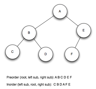
It’s essential to understand preorder and inorder traversal. Let’s take a look at the preorder sequence: A B C D E F
We know that A has to be our root. We don’t know yet if B is the right or left child. Therefore let’s look at the inorder sequence: C B D A F E
Oh, A is on the 4th position, i.e. C, B and D have to be in the left subtree. Therefore B is the left child. Now we have C and D left in the left subtree. Let’s look again at the inorder sequence: C B D A. So C has to be the far left node and because B is the left child D have to be the right child of B.
Now we have to find out where E and F belong. We know that they belong to a right subtree to A. If you look at the preorder sequence you see that E has to be the root of the left subtree. Finally we look at the inorder sequence and see that F is before E. Therefore F has to be the left sub because E is the root and we’re done.

5-8. Present correct and efficient algorithms to convert an undirected graph G be- tween the following graph data structures. You must give the time complexity of each algorithm, assuming n vertices and m edges.
(a) Convert from an adjacency matrix to adjacency lists.
(b) Convert from an adjacency list to an incidence matrix. An incidence matrix M has a row for each vertex and a column for each edge, such that M[i,j] = 1 if vertex i is part of edge j, otherwise M[i,j] = 0.
(c) Convert from an incidence matrix to adjacency lists.

Solution (a)

for y := 1 to n
    for x := y to n
        if matrix[x][y] = 1
            addEdge(x, y)

Which runs in O(n^2) time.

(b)

initialize matrix[m][n]
x := 1
for each entry in list
    matrix[x][from] = 1
    matrix[x][to] = 1

We need O(mn) for initializing the matrix and the loop needs O(m) therefore the algorithm needs O(mn) time.

(c)

for x := 1 to n
    start := None
    end := None
    for y := 1 to n
        if matrix[x][y] = 1
            if start = None
                start := y
            else if end = None
                end := y
    addEdge(start, end)

This algorithm also takes O(n^2) time.

5-9. Suppose an arithmetic expression is given as a tree. Each leaf is an integer and each internal node is one of the standard arithmetical operations (+,−,∗,/). For example, the expression 2 + 3 ∗ 4 + (3 ∗ 4)/5 is represented by the tree in Figure 5.17(a). Give an O(n) algorithm for evaluating such an expression, where there are n nodes in the tree.

Solution

function evaluateTree
    if tree->left-subtree and tree->right-subtree is not a expression
        return evaluate(tree, tree->left-subtree->value, tree->right-subtree->value)
    else 
        if tree->left-subtree is a expression
            left := evaluateTree(tree->left-subtree)
        else
            left := tree->left-subtree->value

        if tree->right-subtree is a expression
            right := evaluateTree(tree->right-subtree)
        else
            right := tree->right-subtree->value

        return evaluate(tree, left, right)

5-18. Consider a set of movies M1, M2, . . . , Mk. There is a set of customers, each one of which indicates the two movies they would like to see this weekend. Movies are shown on Saturday evening and Sunday evening. Multiple movies may be screened at the same time.
You must decide which movies should be televised on Saturday and which on Sun- day, so that every customer gets to see the two movies they desire. Is there a schedule where each movie is shown at most once? Design an efficient algorithm to find such a schedule if one exists.

Solution We can model this problem as a graph problem. Each node is a movie and each edge (x, y) represents a person who wants to watch movie x and y.
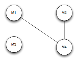
For example: People want to watch movie 1 & 3, 1 & 4 and 2 & 4. Here we can show movie 1 and 2 on saturday and movie 3 and 4 on sunday because there isn’t a connection between movie 1 and 2 and movie 3 and 4. That is, nobody wants to see movie 1 and 2 or movie 3 and 4.
Let’s add an edge between movie 1 and 2 and see what’s happen.

Our last schedule doesn’t work anymore because movie 1 and movie 2 are screened on the same day. We’re looking for a bipartite graph which is discussed early in the book.

5-23. Your job is to arrange n ill-behaved children in a straight line, facing front. You are given a list of m statements of the form “i hates j”. If i hates j, then you do not want put i somewhere behind j, because then i is capable of throwing something at j.
Give an algorithm that orders the line, (or says that it is not possible) in O(m + n) time.

Solution We can save us a lot of time if we model the problem correctly.
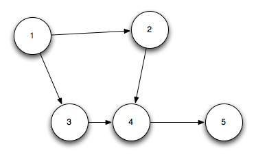
In this example 1 hates 2 and 3, 2 hates 4, 3 hates 4, and 4 hates 5. You can see that we can use topological sorting for this problem which is also described early in the book.

Passionate Programmer: Programming Language and Wage Premium

In the first chapter of Passionate Programmer Chad Fowler talks about the supply of programmers for new technologies and really old ones and wage premiums.

Data

I’ll consider programming language instead of general technology because its too diverse. My first thought was to look at TOIBE which publish a programming language popularity index every month. However, that doesn’t necessary reflect the market demand. So, I looked for other sources and found this blog post which used the indeed jobtrend tool. This gives us a nice idea of trends.

Jan 05 - Nov 11, Jan 09 - Nov 11

Java: +28%, +5%
C: +23%, +1%
C++: -15%, -18%, 
C#: +120%, +24%
PHP: +325%, +140%
Objective-C: +11,000%, +8400%
Visual Basic: -8%, +24%
Python: +610%, +330%
Javascript: +160%, +95%
Perl: +20%, +10%
Ruby: +2,300%, +1,300%
SQL: +30%, +5%
Pascal: -26%, -3%
Lua: +20,000%, +10,000%
Ada: +22%, +16%
Cobol: -45%, -17%
Fortran: -27%, -51%
Erlang: +4,500%, +2,500%
Prolog: -27%, -49%
Haskell: +300%, +225%
F#: +3,250%, +3,250%
Groovy: +4,200%, +3,250%
Scala: +5,500%, +5,500%
Ada: +25%, +17%
CoffeeScript: +2,750%, +2,750%
Clojure: +12,000%, +12,000%
Lisp: +23%, -5%
Delphi: -5%, +7%
ABAP: +15%, +0%

Graphs / Interpretation

Long term and short term growth

I imported the data into Stata, log transformed ( \log(1+x)) it for readability and plotted it with long (6 years) and short (2 years) term growth. Here you can see the whole graph which is quite unreadable beyond C#.

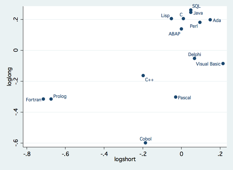
Therefore I split it up into two charts. The first chart contains all languages with less than 100% growth in the last 6 years, i.e. about 12% annual growth on average. This threshold is arbitrary but helps to split the data, so that it is more readable.

For the interpretation: I.e. Cobol is at -0.6 on loglong, i.e. e^{-0.6} -1 \approx -0.45 long term growth. And zero percentage growth means a log value of 0.
We see the expected candidates here, Fortran and Cobol. Ada is quite high which was surprising, at least for me.
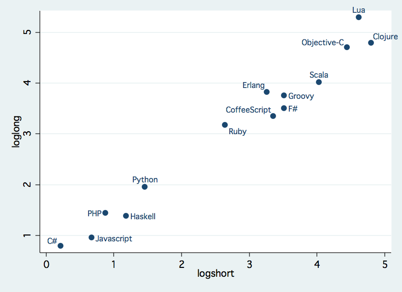
Here’s the other half ot the chart:

Some great newcomers are Clojure, CoffeeScript and Scala. PHP is still strong which surprised me, too.
However, it’s important to consider that e.g. that the demand of Clojure developers increased dramatically but it’s still a niche language.

Salary and growth

At the next step, I took the average salary from indeed for each language and normalized it (\frac{\text{salary} - \text{Average salary}}{\text{Std. Dev. salary}}). If we plot this normalized average salary and the log transformed short term growth we get this graph:

Interpretation: avgsalary indicated the percentage of higher/lower salary to the average (~$88,367) in std. dev (about $12,308). For example ABAP got a avgsalary of about 2, therefore the actual salary is 88,367 + 2 * 12,308 = 111,983.

Also I added a linear regression line which slope is actually significant. (\beta_1 = 0.26 and std. err. of \sigma_1 = 0.095
The data is quite fuzzy so don’t get overly excited. For example the data for ABAP is quite skewed because this also includes e.g. consultants. However, we can see a general trend for higher wages for trendier languages which is to be expected.
If we exclude our outliners, i.e. ABAP, Ada and Visual Basic, we get other data.
Average salary increases to $89,720 and its std. dev. decreases to $8,369 (about a third!). Our estimate gets a lot better (\beta_1 = 0.34 and std dev. \sigma_1 = 0.085). And our graph looks a bit different:

We can see even see some kind of clustering. One with languages with logshort > 3 and then there’s this Java, C++, C# cluster. Quite interesting!

SOPA: Donations and Preferences

Data

I saw on Hacker News a neat website posted called (http://www.sopaopera.org/). The comments stated some hypothesis, e.g. that donations of entertainment and internet companies predict the support or opposition of the SOPA bill.
The data is directly from sopaopera.org which itself aggregates it from various sites.

Graphs & Tests

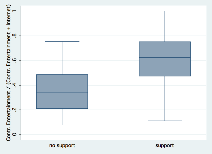
After cleaning the data and importing it into Stata. I looked through it and plotted this box plot which shows how much contributions each group got by entertainment companies in comparison to entertainment and internet company contributions.

In case you don’t know how to read such plot. The thin bars indicate min and max values and the blue box indicates how many people are between the first and third quantile, i.e. 25% to 75% of the population. The line in the blue box shows the median.

You can see that the median for the opposition is about 35% contribution ratio in contrast to the 65% contribution ratio of the supporters. Afterwards, I wanted to test if this difference is significant. In fact, it is highly significant (95%, t = -4.73).

Furthermore, here’s a plot of absolute contributions log-transformed:

The next step is to do a logistic regression to check the prediction quality of each attribute. I regressed with age, party (is_democrat), seniority and quota of entertainment contributions (quota_ent). You can see the results:

 ------------------------------------------------------------------------------
       support |      Coef.   Std. Err.      z    P>|z|     [95% Conf. Interval]  
  -------------+----------------------------------------------------------------
           age |   .0258551   .0358136     0.72   0.470    -.0443382    .0960485
   is_democrat |  -1.252883   .6243361    -2.01   0.045    -2.476559   -.0292067
     seniority |  -.0262688   .0381962    -0.69   0.492     -.101132    .0485943
     quota_ent |   5.839435   1.447732     4.03   0.000     3.001933    8.676938
         _cons |  -1.968467    2.01512    -0.98   0.329    -5.918029    1.981096
  ------------------------------------------------------------------------------

We can see that is_democrat and quota_ent are significant not zero whereby quota_ent is the most significant. This isn’t so much of a surprise.